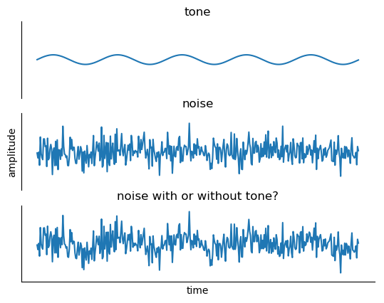
One of the classical experiments of psychoacoustics is the measurement of the lowest sound level at which a tone is heard in the presence of a white noise masker. This sound level is called the 'masked threshold'. In the following example, the masker is played at a fixed level, and the level of the tone can be adjusted. On every repeat of the stimulus, the masker is started first, and a short time later the tone comes in. 

Set the tone to a level at which you can hear it clearly. Introspectively, even though the noise and the tone sum together to a single sound wave, the two sounds sound differently - it is as if two 'objects' were playing at the same time.

Next, find your masked threshold by lowering the tone until you can no longer hear it. What happens for tone levels that are very close to masked threshold? Do you still hear the tone as a 'different thing'? 

Als, is your masked threshold the same if you start with a loud tone and decrease it until it disappears or if you start with an inaudibly quiet tone and increase it until you can hear it?

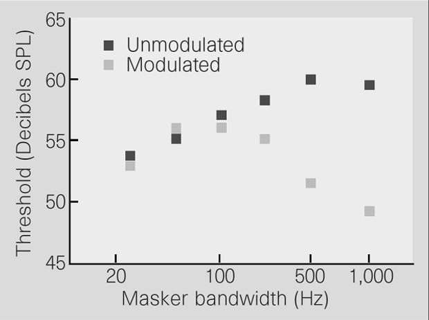
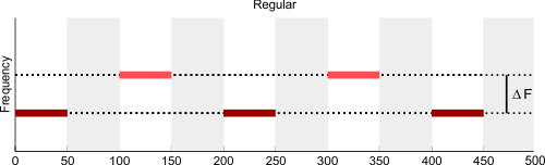
Comodulation Masking Release (CMR) is the decrease in masked thresholds that occurs when the masker is amplitude-modulated. Remember that masked threshold is the lowest tone level at which it can just be heard over the noise. A decrease in masked threshold means therefore that it becomes easier to hear the tone. As a rule, masked thresholds increase with increased bandwidth of the masker, simply because more energy is available for masking. The peculiar property of CMR is that masked thresholds actually decrease with increased bandwidth of the masker when maskers are amplitude-modulated, as illustrated in the following figure.

Here is a sound example illustrating the difference in thresholds of a tone in modulated and unmodulated maskers. Start by setting the threshold with the modulation button in the 'off' position. At that sound level, turn the modulation on. Can you hear the tone now?

While this example illustrates the drop in threshold due to the introduction of the modulation, it is rather the decrease in threshold due to the increase in bandwidth that is the most interesting feature of CMR. However, this dependence is much more difficult to illustrate with the often rather lousy loudspeakers that many computers are fitted with.

The importance of onsets in auditory grouping is illustrated here with the stimuli originally introduced by Darwin and Sutherland (1984) and later studied by Roberts and Holmes (2006, 2007). The sound examples used here are courtesy of Brian Roberts.

The following figure illustrates the basic setup. It shows the spectra of 3 sounds, each with the same pitch, but with different relative levels of the partials. As a  result, the peak location of the spectral envelope varies, as indicated to the right of the figure. The peak location is at the first formant frequency (see Chapter 4 of the book). The sounds have spectral content at higher frequencies as well, but it is irrelevant for the rest of the illustration.

Click on the radio button marked 'original' and then on 'start' in order to hear these sounds. By moving the diagonal slider, you can change the location of F1. The perceptual quality of these sounds is that of a (rather artificial) vowel: when the first formant is low, the vowel is judged to be /I/-like, while when the first formant is high, it is more /e/-like. In the middle, the vowel is ambiguous. In order to experience this demonstration best, position the slider so that the vowel identity is ambiguous.

Next, try the modified sound examples. The first modification is to increase the level of the harmonic at 500 Hz. The result is an upward shift of the formant frequency, and hence a more /e/-like quality of sounds that previously were judged to be /I/. To hear these stimuli, press the '500 Hz louder' radio button. Try to switch back and forth between the original and these modified sounds.

The second modification is to start the 500 Hz harmonic before the rest of the sound. Because its onset is earlier, the 500 Hz harmonic is less fused with the rest of the sound, and its effect on the sound is reduced, moving the perceived quality of the sounds back towards /I/. To hear these stimuli, press the '500 Hz louder, early onset' radio button.

Finally, a 1000 Hz tone is added simultaneously with the 500 Hz tone and is stopped at the onset of the rest of the vowel. This 'captor tone' is expected to fuse with the 500 Hz tone. Since it stops at vowel onset, it is expected to reverse the effect of the early onset of the 500 Hz tone, and to move the perceived quality of the sounds towards /e/ again. To hear these stimuli, press the '500 Hz, early onset, captured' radio button.

The remarkable aspect of this experiment is that the vowel appearing in the three modified stimuli is the same, but its perceptual quality is modified by the context in which it appears. As discussed in Chapter 6 of the book, the reason for the context effect is unclear - it may be due to the properties of neurons in early stages of the auditory system, or alternatively it may represent a high-level interpretation of the sounds by a 'scene analyzer'.

One of the most intensively used paradigm for studying simultaneous sound segregation is the identification of double vowels. The most important result discussed in Chapter 6 of the book is the finding that the introduction of a difference in the pitch of the two vowels improves their identification.

Here is a demonstration of double vowels. The vowels illustrated here are the japanese vowels used by de Cheveigné and colleagues in a series of studies discussed in the book. The software used to generate these vowels was supplied by Alain de Cheveigné.

This demonstration illustrates the inharmonic vowels used by de Cheveigné to study double vowel identification. The software used to synthesize these vowels is courtesy of Alain de Cheveigné.

Here is a demonstration of double vowels. The vowels illustrated here are the japanese vowels used by de Cheveigné and colleagues in a series of studies discussed in the book. The software used to generate these vowels was supplied by Alain de Cheveigné.

UNDER CONSTRUCTION

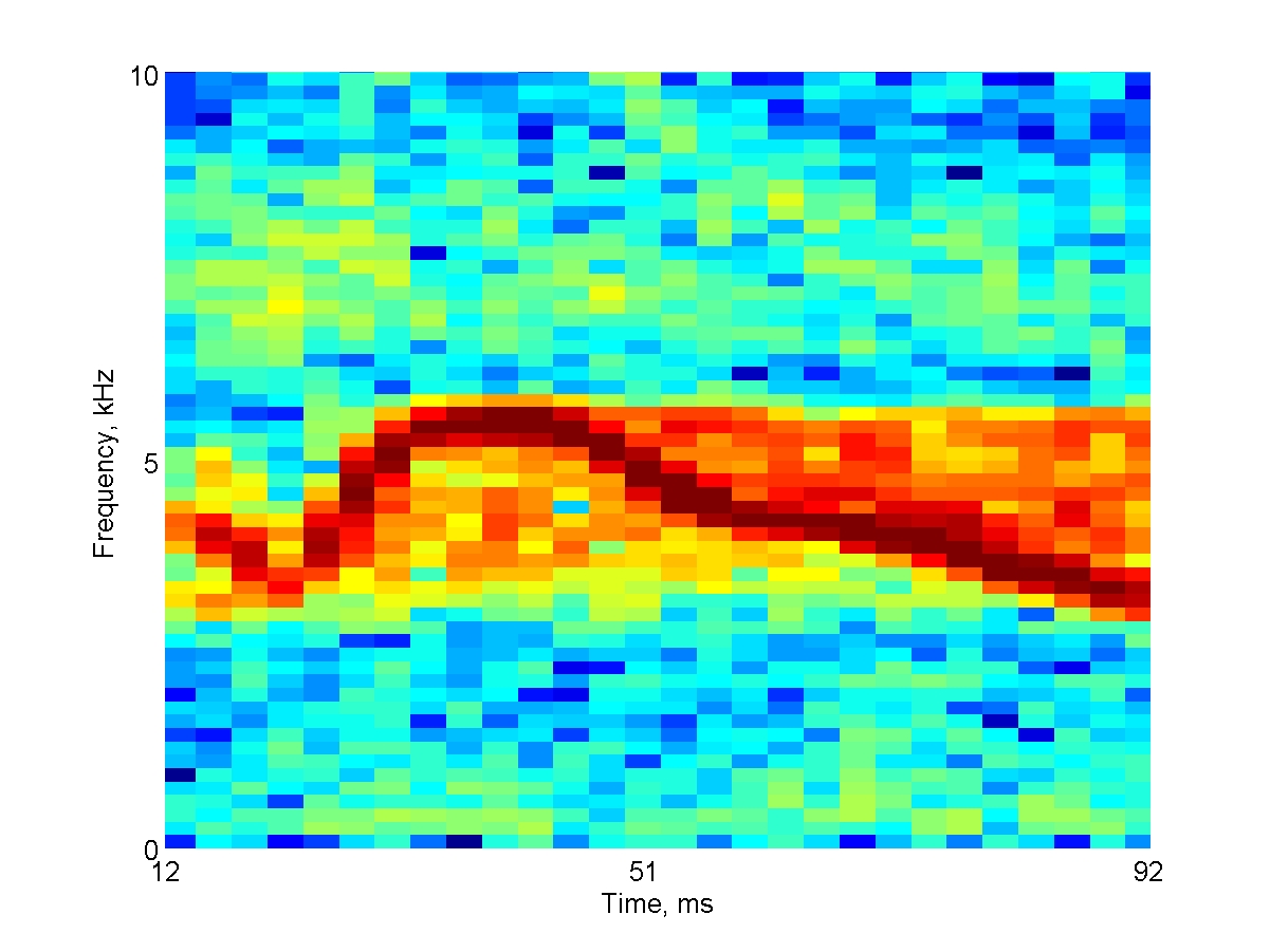
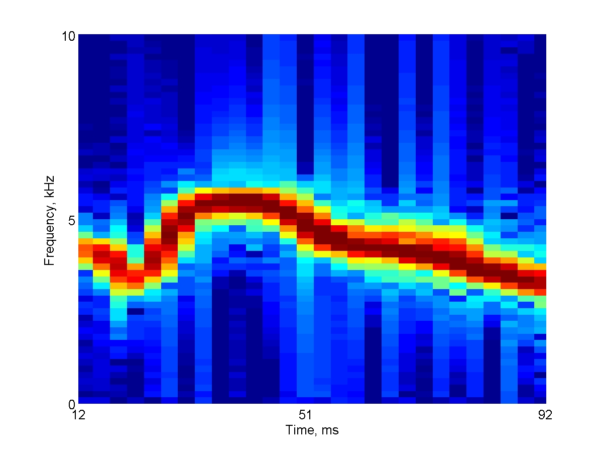
Sounds recorded in nature are almost always mixtures of multiple components. Section 6.3.4 of the book reviews studies (by Bar-Yosef and Nelken) that tested the responses of neurons in cat auditory cortex to bird songs. These songs, which were recorded in nature, contained, in addition to the bird chirps, also echoes and background noise. The sounds have been decomposed into the clean chirps and the background noise. The main result of the experiments (Bar-Yosef et al. 2002, Bar-Yosef and Nelken 2007) was the demonstration that the backgrounds had a very strong effect on the neuronal responses, even in the presence of the much stronger clean chirp.

The following three spectrograms illustrate one of the sounds used in these experiments. You can listen to each sound both at its original sampling rate (44.1 kHz) and at a lower sampling rate (8 kHz). It is much easier to figure out the relationships between the sound and its spectrogram when playing it at the lower sampling rate. The experiments, however, were all conducted with the sounds played at their original sampling rate.

Here's the spectrogram of the full natural sound:

Original Speed:

Slow:

Here's the clean chirp ('Main'):

Original Speed:

Slow:

And here's the noise, which is the difference between the natural sound and the clean chirp. The difference was calculated in the time domain, sample by sample:

Original Speed:

Slow:

When two tones are played alternately at a fixed, slow, rate, the result is a simple melody consisting of the two alternating tones. However, if the rate of presentation is fast enough and the frequency separation between the two tones is large enough, the melody breaks down into two streams, each consisting of tones of one frequency.

The following demonstration illustrates streaming. The horizontal slider changes the rate of presentation, while the vertical slider changes the frequency difference between the two tones. Start at the slowest presentation rate (leftmost position of the horizontal slider) and the smallest frequency difference (lowest position of the vertical slider). Now move to the fastest presentation rate and the largest frequency difference. What happens? Try to map the range of parameters in which the splitting of the sequence into two streams occurs.

This is yet another example of streaming, using the 'galloping', or 'ABA' rhythm paradigm. The two possible perceptual states of this sequence are illustrated in the figure below (this is Fig. 6-11 of the book). When the repetition rate is slow, or the interval between the two tones is small, the sequence is usually perceived as a 3-note melody with a galloping rhythm. At faster rates, or when the interval between the two tones is large, the sequence breaks down into two streams, the upper one at half the repetition rate of the lower one.

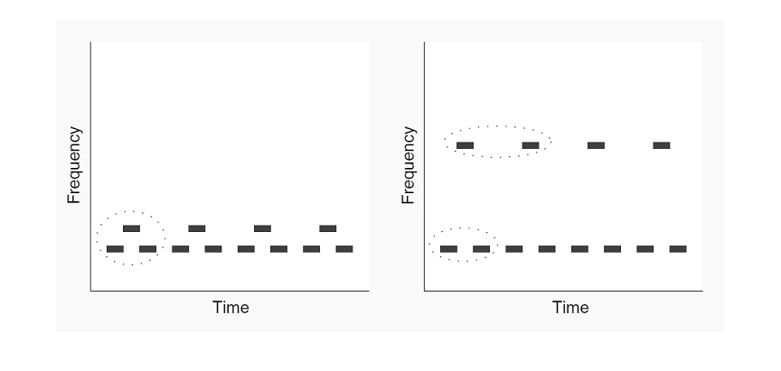
You can experiment with these sounds below. Start at slow repetition rates and small frequency intervals, then move to faster rates and larger intervals. Try to locate the combinations that result in the perception of two streams. Can you hear the streams separate and merge back?

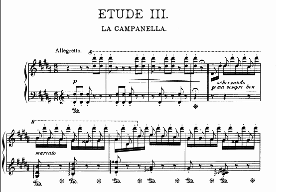
Streaming has been used by classical composers as a way of creating simultaneous multiple melodies with an instrument that can produce only one note at a time. The standard examples come from Bach's compositions for violin solo.

Here's a less standard example, coming from a rather well-known piece for piano. As a rule, pianists don't need tricks to produce multiple melodic lines. The la Campanella etude is an exception - Liszt wanted to mimic Paganini's violin on the piano, producing on the way one of the most difficult pieces in the piano repertoire. It is one the Grandes études de Paganini composed by Franz Liszt and published in 1851. An earlier version figures in the Études d'exécution transcendente d'après Paganini from 1838.

There are a fair number of performances of these etudes on YouTube. Enjoy the viruosity!

Here's an illustration of streaming by amplitude modulation. The sounds you will hear are all sinusoidally amplitude-modulated pure tones. The carrier frequency is always at 6 kHz. The galloping rhythm is produced by an 'A' tone that is modulated at a rate of 100 Hz  while the modulation frequency of the 'B' tone can be changed from 106 Hz to 800 Hz.

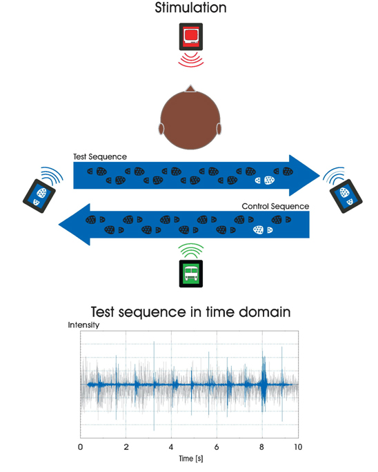
Winkler et al. (2003) demonstrated that it is possible to evoke MMN with natural stimulation (well, almost natural). The sound and the illustrations below are courtesy of Istvan Winkler.

The subjects were busy watching and listening to a movie. They also heard background noise from the street, over which 11 steps were heard. Either the second or the one but last step were different from the others, and the MMN was calculated as the difference between these two conditions - presumably, when the different step was at the end of the sequence, it was detected as a deviant relative to the others.

In the illustration below, the footsteps are plotted in blue, the street noise and the movie in gray. The deviant step is at about time 8 s.

Here's the resulting MMN:

The sound example below is the deviant condition:

Humans show evidence of being able to preattentively extract rather complex rules governing a stimulation sequence. One of the most extreme examples in the literature comes from a paper by Paavilainen, Arajarvi, and Takegata (2007), as described in chapter 6 of the book.

Here is a sequence of sounds following the rule used in that paper. It is composed of four possible stimuli: a high frequency tone and a low frequency tone, each with either a short duration or a long duration. Can you find what is the rule that govern the sequence?

Study now the figure below. It illustrates the rule governing the sequence - stimuli marked by S follow the rule, stimuli marked by D do not (this is NOT the sequence you have just heard, which follows the rule without any exception).

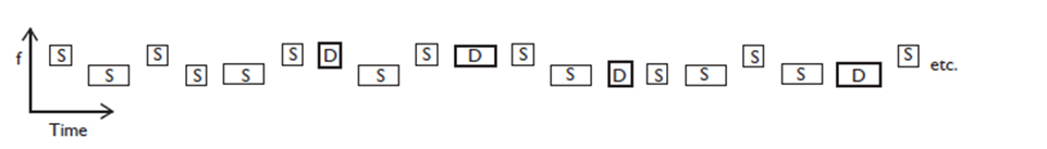
Can you figure out what is the rule governing the sequence now?

The rule underlying the sequence is the following: a short tone is followed by a low tone (which can be short or long, with probability 0.5 each), and a long tone is followed by a high tone (which can be short or long, with probability 0.5 each).

Here's the sequence again. Can you follow the rule now?

Paavilainen et al. (2007) reported that even subjects who were instructed about the structure of the sequence could not reliably indicate deviations from the regularity. Nevertheless, they had a significant MMN. Thus, somewhere in their brain, the rule governing the sequence was presumably extracted, and deviations from the rule were detected.

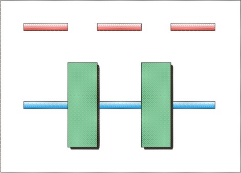
The "Law of Continuity", one of the "Gestalt rules" thought to govern perception,  stipulates that our mind will tend to interpolate or extrapolate perceptual "objects" if the edges of the objects are obscured. A visual example is shown in in the graphic here. The red line, however, is obviously broken in two as you can see the gap. However, most people would see the blue line as continuous, assuming that it continues behind the green boxes. 

The audio example below illustrates a similar effect in hearing. Short pure tone "beeps" occur repeatedly at short, regular intervals. These beeps continue unaltered throughout the sound example, but as the beeping continues, a pulsed noise slowly grows and then fades in amplitude. The noise pulses have been arranged so that they fall in the gaps between the beeps. A few seconds into the sound example, the noise will have become loud enough to cover up ("mask") the gaps in the beeps, so that the beeps are heard as a continuous tone. 

(If you want to download the mp3 of the demo, right-click this link and choose "save as").

The following demo explores the effect of temporal regularity, or rhythmicity, on stream segregation. It uses the stimuli used in the study by Rajendran and colleagues (2013 JASA-EL).

This demo works well with recent versions of Google Chrome, Firefox and Safari.

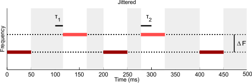
Rapidly alternating (ABAB...) tones are usually perceived, at least initially, as a single "trill"-like sound, but after a while the single auditory stream may appear to break into two, with either the A-A- or the -B-B sequence dominating the percept, and the other tone sequence becoming a "background" sound. The wider the frequency separation, the quicker generally the break-up into two streams. Here are two example ABAB sequences with frequency separations of either 1 semitone (heard by most as one stream throughout) or 10 semitones (heard by most as two streams after only a second or so).

1 Semitone Sequence

10 Semitones Sequence

Wider frequency separation is not the only factor that increases the likelihood that two streams are perceived instead of one. Another factor which seems to play a role is temporal irregularity. Here you can try 3 second long sequences of varying frequency separation, and you can also introduce varying degrees of temporal irregularity ("jitter") into the higher frequency tone sequence.

The five jitter values on offer replicate the values used in the experiment by Rajendran et al., in which temporal jitter was chosen from a uniform distribution around the "expected" timing of each B tone once every 200 ms.

What to try: Start the sequence with a 4 semitone separation and zero jitter. If your hearing is like mine, most of the time you will hear that as a single stream, of alternating high and low notes. Now switch the RMS jitter from 0 to the maximum, 18.48 ms. If your hearing is anything like mine, your percept should relatively quickly flip to have two different streams, one stream of regularly spaced low pips and one stream of irregularly spaced high pips. And when you switch back to zero jitter, the two streams may fuse again into a single low-high-low-high pattern. You can experiment with larger or smaller frequency steps. Larger frequency steps should make two stream percepts more likely even if there is no jitter. Larger jitter values should make two streams more likely even if the frequency separation is relatively large.

 

delta F (semitones)	RMS Jitter (ms)
1	0
4	2.31
7	4.62
10	9.24
	18.48
Play Sound Sequence