Many objects in nature can be thought of as "mass-spring-systems" because they are composed of objects which have inertial mass as well as a spring like stiffness. It is natural for mass spring systems to enter into sinusoidal oscillation. These oscillations may create vibrations of the surrounding air (i.e. periodic sounds), as described under "sound propagation" below.
This figure is an animated version of Figure 1-1 of "Auditory Neuroscience" 

testing

A guitar string, plucked at the centre, will be stretched into a triangular shape before you let it go. Once you let it go it will vibrate in a "triangular sort of way". The thing about its motion is that it can be thought of as a superposition of simple harmonic motions, with harmonically related frequencies, as shown here. The "more or less triangular" vibration in the lowest panel arises as a weighted sum of the three modes of vibration shown above it. 

This animation complements Figure 1-3 of "Auditory Neuroscience". 

In the previous animation you have seen how a plucked guitar string will vibrate at numerous "modes of vibrarion" at once, and therefore produce sound at many harmonically related frequencies ("overtones"). Just to show that these modes of vibration are real, here a little youtube video by nicogetz, where he placed a camera phone inside his guitar and then played a tune. The camera phone is too slow to pick out all the details of the motion of the strings (the phone will collect somewhere around 40 to 70 frames a second, while the highest harmonics of the motion of the strings may vibrate at several thousand frames a second) but the result is that only some of the modes of vibration will be "aliased" by the video to become visible to the naked eye. Nevertheless a beautiful illustration to show that modes of vibration are a feature of sound sources.

This javascript app calculates a spectrogram from the input to your computer's microphone. (You may have to adjust the sensitivity a bit.) A spectrogram is in some ways similar to the activity pattern that auditory nerve fibers send to your brain, so you can use this spectrogram app to visualize what various sounds or speech would "look like" to your brain. You can pause the spectrogram by clicking on it.

Spectrograms can be useful to visualize the frequency content of sounds, and to give a rough-and-ready approximation of the activation pattern a sound is likely to generate across the auditory nerve array. For classroom demonstrations, or just to explore sounds, it's nice to have a piece of software which will record sounds from the microphone of your computer and will display the spectrogram online on the computer screen. One nice freeware program for that purpose was created by a company called Visualization Software, but their website seems to have gone off air (perhaps the company ceased to exist). This screenshot shows the program in action, visualizing the spectrogram of me pronouncing the vowels /a/-/e/-/a/-/e/-/a/ . The change in formants as well as the harmonic of the vowels are showing up clearly.

As it is a very nice and useful little freeware program I am making the installation file available here. It's a Window's program. It comes with absolutely no warranties! My virus checker thinks it's kosher, and when I've used it for lectures and classroom use it has always performed beautifully (kudos to the folks from Visualization Software!), but use it at your own risk (and since I am not the author, please don't send me any bug reports - I would not know what to do with them).

Sound propagates as a longitudinal wave. Although air is relatively light, it does weigh something. Air is also "elastic": if you try to compress it, it will push back. Given that air has both elasticity and mass, you can imagine the air around you as being made up of little "lumps of air", where each lump is connected to the next lump by an elastic spring.

If an object (e.g. the small bar at the left edge of the animation below) pushes against such a column of air, it compresses the air immediately next to it. This compression propagates away from the object as a "compression wave", as each lump of air pushes against its next neighbor. If the object then returns to its original position, it draws the air back, creating a "rarefaction wave" which follows the compression wave.

The animation here, essentially an animated version of Figure 1.17 of "Auditory Neuroscience", illustrates this.

In the "free field" (meaning in the absence of obstacles that might interfere with wave propagation), sound waves will spread out in all directions, like spheres radiating out from the source at the speed of sound.

Clearly, as the radius of the spheres gets larger, the amount of acoustic energy in the sound gets "stretched thinner and thinner" over the expanding surface of the sphere. Given that the surface of a sphere is proportional to the square of its radius (A = 4⋅π⋅r2), the energy in the sound wave that would impinge on a fixed small area (e.g. an ear drum) therefore declines with the square of the distance from the source.

This relationship between sound intensity and distance from the source is known as the inverse square law.

Note that in closed rooms where considerable amounts of sound energy may be reflected back from walls, floor or ceiling, the inverse square law usually does not hold.

Drag The Points On the Graph to Test Your Hearing

Put on headphones. Drag the points down until the sounds are only just audible.

What to expect:

This little demo is not too unlike the standard audiometric test known as a pure-tone audiogram. We present pure tones of different frequencies at different sound levels, and adjust their level until they become inaudible in order to measure the "threshold". Obviously, the quieter you can make the sound and still hear it (i.e. the lower your threshold) the better. You can use the buttons beneath the graph to switch from the left to the right ear. You may find it interesting to compare your left and right ears and see if they are equally sensitive. 

Note that, unlike in a clinical audiogram, here we are plotting the sound intensity simply as "dB full scale", meaning decibel below the maximum output that the computer can produce given how powerful your soundcard or amplifier, what volume settings it has, and how sensitive and accurate your headphones are. Obviously, if your computer or headphone amp has its volume turned down then your thresholds may seem lower than they would otherwise be. Similarly, if you are sitting in an environment with background noise, that noise will mask the quietest tones and your threshold will again seem higher than it really is. To do an audiogram as a clinical test, an audiologist would:

1. put you in a sound proof chamber to minimize background noise, and 
2. use calibrated headphones, to be able to work out how many dB SPL (sound pressure level) or how many dB HL (hearing level) the dB full scale correspond to. 

Note that, when an audiogram is expressed in dB SPL or dB full scale, then you would expect it to be "U shaped", meaning that your thresholds for sounds between 1000 and 4000 Hz should be the lowest, and thresholds should increase for frequencies which are much lower or much higher than that range. That is because our outer and middle ears have their own resonant and acoustic impedance matching behaviors which make them very good at transmitting 1-4 kHz sounds to the inner ear, but much less good at transmitting higher or lower frequencies. So if we want to make a 100 Hz tone and a 4000 Hz tone that are meant to sound equally loud, then we actually have to make the 100 Hz tone physically more intense. This "iso-loudness curve" shows that effect:

In clinical audiograms, expressed in dB HL, the frequency dependent changes in sensitivity of the human auditory system are subtracted out, so a clinical audiogram should be fairly flat, rather than U-shaped, with values near zero. Unless there is something wrong. What healthy and unhealthy clinical audiograms look like you can find out on the next page.

Clinicians measure sound intensity in dB HL (decibels Hearing Level), i.e. dB relative to the quietest sounds that a young healthy individual ought to be able to hear.  In a clinical audiogram test, pure tones between ca 250 and 8000 Hz are presented at varying levels, to determine a patient's pure tone detection thresholds (the quietest audible sounds) in the left and right ear. Thresholds between -10 and +20 dB HL are considered in the normal range, while thresholds above 20 dB HL are considered diagnostic for mild, moderate, severe or profound hearing loss, as shown here:

Particular causes of hearing loss will be show up in the clinical audiogram in characteristic ways.

Conductive Hearing Loss 

Conductive hearing loss comes about when the transmission of sound to the inner ear is impaired, perhaps due to impacted ear wax (cerum), an ear infection (otitis media with effusion or OME), or calcification of the middle ear ossicles (otosclerosis). Conductive hearing loss tends to a loss of sensitivity across the entire range of frequencies, most commonly in one ear only. A so called "bone conduction test", where sound is delivered as vibration to the skull rather than as airborne sound to the ear canal, can be used to confirm a suspected conductive hearing loss.

(image source: US Occupational Health Administration)

It is often possible to treat conductive hearing loss by removing the cause of the physical obstruction.

Sensory-Neural Hearing Loss

By far the most common cause of sensory neural hearing loss is damage to sensory hair cells in the cochlea. The outer hair cells in particular are very fragile, and can be damaged by exposure to excessively loud sounds, or they may simply "wear out" in old age. In rarer cases, hair cells can also be damaged by certain chemicals (such as high doses of aminoglycoside antibiotics).  Sensory-neural hearing loss can also be caused by damage the auditory nerve, but conditions producing such damage are relatively rare, while noise damage or age related hearing loss are very common complaints. Central hearing loss (due to damage to the central nervous system) is rarer still. Noise damage or age related hearing loss tends to produce characteristic deficits as shown in the audiograms here below. Unlike conductive hearing loss, which can often be cured, sensory-neural hearing loss is in most cases irreparable, and treatment will aim to make the best use of those auditory structures that remain in tact, perhaps by boosting sensitivity through a hearing aid, or, in severe cases, by trying to bypass dead sensory hair cells with cochlear or brainstem implants.

Noise damage

Because our outer and middle ear transmits frequencies near 4 kHz very efficiently, hair cells that are tuned to frequencies near 4 kHz are particularly vulnerable to noise damage. Therefore, audiograms of patients with noise damage often have characteristic 4 kHz notches, as shown here:

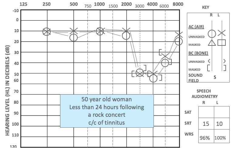
(image source: audiologyonline.com)

Age-related Hearing Loss (Presbycusis)

Even if we avoid exposure to very loud noise, the ear's outer hair cells may also simply wear out as we age, leading to age related hearing loss. In this condition, high frequency outer hair cells tend to die off before low-frequency ones, possibly because the high frequency outer hair cells have to work harder if their job is to amplify acoustic vibrations on a cycle by cycle basis. Consequently, patients with age-related hearing loss often have normal sensitivity at low frequencies, but progressively poorer sensitivity for higher frequencies, as shown here:

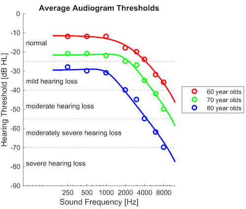
If you are curious about what the effect of such age related hearing loss would be, try our Age Related Hearing Loss Simulator.