Spatial Hearing
Spatial Hearing
Under optimal conditions, humans can, even with their eyes closed, localize the direction of sound sources to an accuracy of a few degrees. That is not a trivial feat. Just try to imagine you had to work out the location of all the boats, fish, swimmers, etc, swimming about in Sydney harbour purely by analysing the pattern of waves and ripples on the surface of that waterway. That would be difficult enough to do if you can observe the waves across the whole body of water, but of course your auditory brain solves a similar feat by observing the waves at only two points in space: your two ears. Chapter 5 of "Auditory Neuroscience" discusses spatial hearing, the cues that we use to localize sound sources, and the neural mechanisms involved in processing this information. The following web pages provide additional material to further explore this topic.
Fox hunting by sound localization
Fox hunting by sound localization
This small extract of the "Yellowstone" nature program from the BBC shows a fox which is using his sound localization ability to hunt prey animals that are concealed under a cover of snow.
Acoustic cues for sound location
Acoustic cues for sound location
This figure shows acoustic cues to sound source direction. It is a color version of Fig. 5-2 of "Auditory Neuroscience", and is based on acoustic recordings from my own ears carried out by Prof Doris Kistler at the University of Wisconsin at Madison.
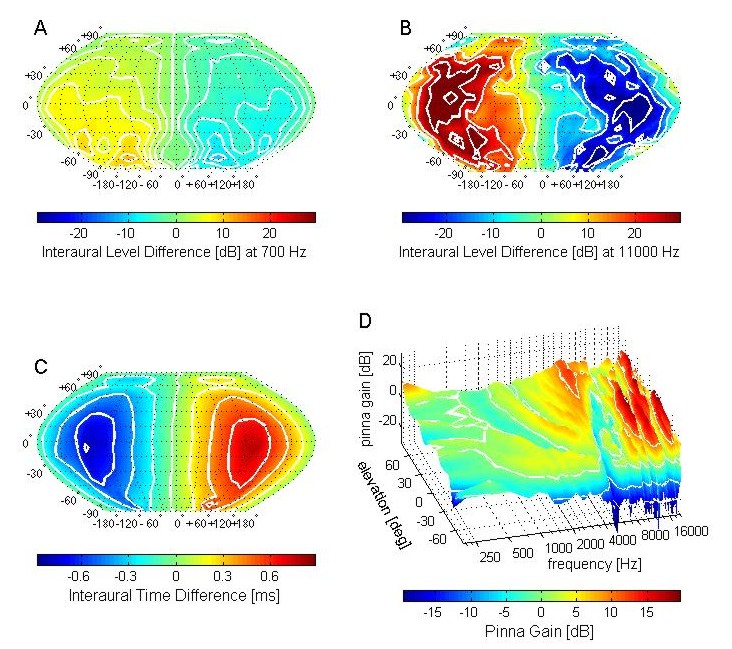
The data are shown as spherical map projections, with my head at the centre of the sphere, and the interaural cue values shown by the color codes for the corresponding sound source directions in azimuth and elevation. A and B show interaural level differences (ILDs) in decibel. As you can see, ILDs are highly frequency dependent, i.e. high frequencies (say near 11 kHz, panel B) can generate large ILDs of 30 dB or larger, while lower frequencies (say near 700 Hz, panel A) generate ILDs of well below 10 dB.
ILDs are also significantly affected by the geometry of the head, outer ears, and shoulders, which is why the patterns of the ILDs are much more irregular than the Interaural time difference (ITD) patterns shown in C. ITDs are nearly spherically symmetric around the interaural axis, are much less frequency dependent, are maximal for positions right off to one side of the head, and never exceed values of 700 microseconds or so.
ITDs and ILDs are both valuable cues for localizing sound sources, but even individuals who are deaf in one ear can sometimes localize sounds in space with some degree of accuracy. These judgements are thought to be based on monaural spectral cues (shown in D for sound source locations right in front, 0 degrees azimuth, at various elevation). Spectral cues arise because the outer ear filters sounds in a manner that depends on the angle of incidence of the sound waves, creating patterns of peaks and notches in the high frequency end of the sound.
The Jeffress Model - Animation
The Jeffress Model - Animation
The Jeffress Model has long been a popular model for trying to exlpain how the mammalian Medial Superior Olive (MSO) or the bird nucleus laminaris may extract interaural time differences for sound localization. The Jeffress model posits a "delay line and coincidence detector" arrangement which is illustrated in the animation shown here. The animation nicely conveys the appeal of the Jeffress model. Due to a systematic delay line arrangement and a requirement for precise synchrony in the activation of MSO neurons, different parts of the MSO become sensitive to sounds from particular directions. But note that the cartoon shown here is in many ways "biologically naive", oversimplifying the anatomy and physiology. Whether the Jeffress model, such as it is shown here, is really a good description of the operation of the mammalian MSO is becoming increasingly controversial.
(Note: the video contains no sound).
Acknowledgement: this video is from the web page of the laboratory of Prof. Tom Yin of the University of Wisconsin, one of the pioneers of research on the physiology of the mammalian MSO.
Widely Separated Ears
Widely Separated Ears
Sound localization relies heavily on interaural disparities (i.e. differences in the signals received in the left and right ears), and these differences are larger, making sound localization easier, if the two ears further apart.
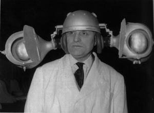
Devices which artificially separate the separation between the ears, for example with suitable tubing, can therefore make it easier to pinpoint the direction of sound sources. An impressive example of such a device, the "hearing throne" of the Oldenburg Hearing-Gardens, is pictured here:
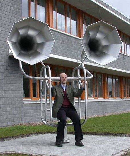
Also, if the ears are offset vertically rather than aligned horizontally, this may help judge the elevation of a sound source. The following images, from the collection of the Waalsdorp Museeum in the Netherlands, are from an era when radar was not yet widely available, and show attempts to use this fact to develop devices to locate enemy aircraft:
Further examples of devices intended to improve spatial hearing, including this wonderful portable contraption, can be found at http://www.damninteresting.com/can-you-hear-me-now
Binaural Cues and Cue Trading - Audio Demos
Binaural Cues and Cue Trading - Audio Demos
This page has little animations illustrating the two major binarual cues for sound source direction: Interaural Time Differences (ITDs) and Interaural Level Differences (ILDs).
You will need to listen to the sound tracks of the videos using headphones. To perceive the effects, you need to have good hearing in both ears. If you have a temporary or permanent hearing loss in one ear, the demos won't work for you. (sorry!) They also may not work if your headphones or the sound card on your computer are poor quality. A number of laptop sound cards in particular "cut corners" when it comes to reproducing some temporal features of sound with great accuracy, which will cause these demos not to work correctly. Note also that many wireless bluetooth headphones are not regenerating ITDs properly, so if you use wireless headphones the ITD part of the demo may not work properly either. Also if you have the headphone the "wrong way 'round" (i.e. the transducer that is meant to go to the left ear connected to your right ear) then the sound may appear to come from "the wrong side".
What to observe
The demos below show and play short 500 Hz tone pips which vary either in ITD only, or in ILD only, or in both ILD and ITD at the same time.
The first demo shows variation in ITD alone, starting with the left ear leading by 0.4 ms, then the ITDs shift in steps of 0.2 ms until the right ear leads by 0.4 ms, and then they shift back. If the demo is working as it should, you will hear the sound source appear to move from a place somewhere slightly to the left to somewhere slightly to the right.
Varying ITDs Only
The second demo keeps ITDs constant at zero, but changes ILDs, so that the left ear sound is initially 6 dB more intense. The ILD then shifts in 3 dB steps to the right, and back again. These ILDs are exploited in stereophonic music, and you will not be surprised that they can appear to shift the sound source to the left or to the right, but you may find it peculiar that either changing ITDs or changing ILDs can lead to similar perceived changes in sound source position, even though they do very different things to the sound.
Varying ILDs Only
Of course, for normal, free-field sound sources, ITDs and ILDs covary, i.e. the sound will be both earlier and more intense in the nearer ear. The most natural situation is therefore the one shown in the 3rd demo, where ITDs and ILDs vary together. If your ears are like mine, then the impression of a moving sound source in this 3rd example will be clearer and more compelling, and the source will seem to move over a wider range, than in the first two examples.
Varying ITDs and ILDs together
With artificial headphone sounds we can also make ITD cues and ILD cues oppose each other, i.e. the sound might start earlier in the left ear but be louder in the right. With such conflicting cues, our brains tend to perceive "compromise" positions near the midline, a phenomenon described as "cue trading". This is illustrated in the fourth example. Here, the sound source should appear to move much less than in the 3rd, and possibly also less than in either the 1st and 2nd examples.
Trading ITDs off against ILDs
Individuals tend to vary somewhat in how sensitive they are to ITDs, and if your sensitivity to ITDs is very low then you may not hear any movement in the first example, and not much difference in the 2nd to 4th examples. (However, it is also possible that the sound card or sound software on your computer is cutting corners and not reproducing ITDs accurately, as seems to be the case for example on my Acer Aspire 1810 laptop). In contrast, if you are very sensitive to ITDs, you may find that the first example gives more compelling movement than the 2nd. Your individual sensitivity to ITDs will affect how much movement you hear in the 4th example, if any, and in which direction.
ILD / ITD practical
ILD / ITD practical
Here below you can find the Matlab source code for a program authored by Matthieu Lesburgueres and Jan Schnupp which you can use to run a psychoacoustic experiment to measure your own sensitivity to ITDs and ILDs.
-
Click HERE to download a zip archive of the Matlab code source.
-
Unzip the content into a folder of your choice.
-
Start Matlab and change the matlab working directory to the folder where you have copied the content of the zip file.
-
Put on headphones, make sure the volume of your soundcard is not set very loud.
-
To start the experiment, run "Experiment.m"
When you got that far, click on Collecting ILD data below for instructions what to do next.
Collecting ILD data
Collecting ILD data
When you launch Experiment.m you should obtain a window which looks like this:
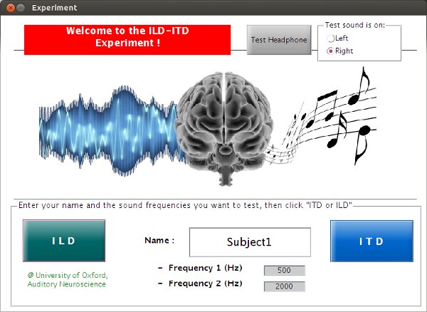
Before you run the experiment, we need to check that the computer knows which sound channel maps to which ear on your headphones. Put your headphones on and click the "Test Headphone" button on the top right of the "Experiment" window. You should hear a short noise burst in one ear only - most likely, but not necessarily the right ear. If the sound was on the left rather than the right, don't worry, just make sure the radiobutton at the top right is set to indicate which side you heard the sound on.
Now you are ready to run the experiment. Enter your name or nickname in the box in the center (this will be used to label data file names and graphs generated as you run the experiment) and choose two sound frequencies at whcih to measure your binaural cue sensitivity. We suggest 500 Hz and 2000 Hz as good frequencies to try.
Question: would you consider 500 Hz and 2000 Hz low frequencies, or high? Bear in mind that the human auditory system operates over a freqency space of ca 50-16000 Hz, but that frequencies are represented in a roughly logarithmic manner, i.e. the 100 Hz frequency span 100-200 Hz is one octave, while the 8000 Hz wide span from 8000-16000 Hz is similarly also only one ocatve.
Once you have entered your values for Name, Frequency 1 and Frequency 2, click ILD to launch the first part of the experiment. Listen carefully because the first sound for you to listen to will start playing very soon after you clicked ILD.
A pop-up window will appear which looks like this:
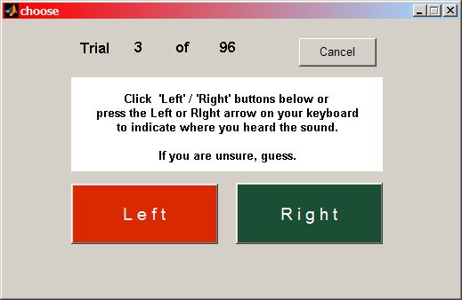
Indicate whether you heard the last sound as coming from the left or the right. Note: many fo the sounds will sound very close to the center, while others will be more clearly on one side or the other. So sometimes you may find it hard to tell. In those cases your answer should be "your best guess". That your best guesses may be wrong some of the time when the tested ILD values get small is part of the experiment.
You can indicate your decision either by clicking on the "Left" or "Right" buttons, or by pressing the Left or Right arrow keys on your computer keyboard. When you have indicated your decision for the last sound presented, the software will automatically present the next sound after a short delay, so keep listening attentively until you have completed all the trials. The software will present high or low sounds of varying ILDs in a random order. Note that, just as it is quite possible for a fair coin to come up "heads" on five or six coin flips in a row, you may also have quite large "runs" of successive sounds on the left or the right.
I personally find it helpful to rest two fingers above the left and right arrow keys on my keyboard, then listen with my eyes closed, and run through the trials in fairly quick succession. If you are doing this for the first time, you may want to do a test run of only about 20 or so trials to become comfortable with the procedure, then stop the experiment by clicking "Cancel" above, and then restart it by clicking "ILD" again on the main window.
Once you are comfortable with the procedure, run through a whole set of trials. The software will automatically generate a plot of your responses in this run. How you should interpret those data is explained in the next section.
Interpreting the ILD data
Interpreting the ILD data
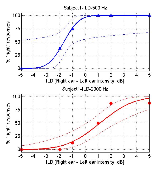
When you have completed your trials the program will generate a plot of your results for you, which should look more or less like this:
If you are doing these exercises as part of a taught class, you should consider making a print-out of these result graphs so that you can show them to your instructors if necessary. (There should be a File | Print menu on the top left above the figure).
The triangular or circular symbols show how often you clicked "right" for the ILD value given on the x-axis. The continuous line is a "cumulative Gaussian" sigmoidal curve fitted to your data by the software. Fitting curves like this is a good way of estimating the "underlying psychometric function" (i.e. the function that describes your sensitivity to changes in a particular sensory parameter) from the data sample we obtained.
Question: On the psychometric functions you obtained, which ILD values are associated with 50% right responses? Which ILD value would you expect to be associated with 50% right?
Psychometric curves are useful for determining how sensitive you are to ILDs. The steeper the slope of the sigmoid, the smaller the change in ILD required to produce a "noticeable" difference in your % right judgments. However, people rarely report sensory performance as slope values (%right/ dB). Instead, they tend to report "thresholds", i.e. changes in ILD which are just large enough to raise the %Right judgments from 50% (completely random guessing) to some "threshold performance level".
Exercise: Choose a threshold level (75% correct might be a good choise) and determine the corresponding ILD threshold for the two frequencies tested. Make a note of these ILD thresholds.
The thresholds obtained for the two frequencies may be very similar, or somewhat different. Do you have a feeling for whether they are "meaningfully different"? There are really two aspects to this question: 1) is the difference "substantial" (physiologically significant, and 2) do you think it might be statistically significant? For the first part you will need to use your judgment - there is no generally accepted way of deciding how big is big. But if the difference is not statistically significant, then any observed difference in thresholds for the two frequencies may not be real.
However, to answer the second part of this question rigorously would require a suitable statistical test, for example some type of "bootstrap". The statistical techniques needed to do this properly are somewhat beyond the scope of this practical. However, you may be able to gain some intuition about this if you think about the problem in the following manner: Your "true" psychometric function will specify: for each particular ILD, the probability that you will report the sound as coming from the right. The experiment cannot measure this probability directly, only estimate it from the frequency of actual right responses in a quite limited number of trials (here about 8 for each ILD tested). Let's say the true underlying probability for a particular ILD was 75%. Testing that ILD would then be a bit like flipping a biassed coin that has a probability of landing "heads" on 75% of trials. Would it be impossible for such a biased coin to produce, say, only 50% heads in a short run of only 8 trials? If you think this through you will probably appreciate that the % right scores observed in this very short experiment are only very rough estimates of your true psychometric function. You may also have wodered what the think broken curves on teh plots represent. These are 95% confidence intervals for the psychometric functions fitted to your data. The algorithm that fitted the sigmoids is clever enough to appreciate that the sigmoid it produced is only an estimate, and that the true underrlying function could be fairly different from that "best estimate". So when you compare the data obtained at the two different frequencies, you could ask yourself, would it be unreasonable to suspect that the data points in the top graph come from the confidence interval plotted in the lower graph, or vice-versa?
Question: Would you consider your sensitivity to ILDs essentially similar, or substantively different, for the two frequencies you tested?
Evaluate the usefulness of ILDs as localization cues
Evaluate the usefulness of ILDs as localization cues
Using the methods described in the previous sections, you should by now have obtained estimates of your own ILD sensitivity at two different test frequencies (500 and 2,000 Hz if you ran with the suggested values). Your ILD thresholds in dB may or may not have been very similar for the two frequencies. However, ILDs are a cue to sound source direction. Source directions are not specified in dB! To localize sounds in space, your brain needs to "translate" ILD values to angles relative to the inter-aural axis. To see how useful a particular ILD would be, say, for detecting a change in sound source direction away from "straight ahead" (zero degrees azimuth) we need to know what ILD values are normally associated with different sound source directions for different sound frequencies. The graph below shows ILDs measured as a function of sound source direction measured in an adult male with small microphones inserted in the ear canal. ILD values are plotted for a number of frequencies and sound source directions (azimuthal angles).
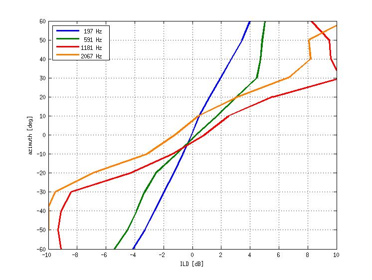
This graph is rather busy, but you will hopefully appreciate that the slope of these graphs near zero is different for different frequencies.
At frequencies close to 500 Hz, the slope is equivalent to approximately 7.35 degrees / dB, while at frequencies near 2000 Hz the slope is closer to 4 degrees / dB. Using these slope values as well as the ILD thresholds you have estimated for those frequencies, calculate your estimated "minimum audible angles (MAAs)", i.e. the changes in source direction that would correspond to the ILD thresholds that you have estimated earlier. Make a note of the MAAs.
Does a smaller MAA mean better or worse spatial hearing?
Did you obtain a smaller MAA at the higher or lower frequency?
Collecting and Interpreting ITD data
Collecting and Interpreting ITD data
Once you have collected, interpreted and evaluated your ILD data, go back to the software's main screen, and collect ITD data by clicking on the "ITD" button
 .
.
The software will once again play sounds of high or low frequencies and ask you to indicate whether you heard them as on the left or right by muse clicks or keyboard arrow keys. Run through the trials using the same procedure as when you collected the ILD data. Note: most people find it very difficult to hear ITDs for high frequencies as lateralized to the left or right. So you will probably hear most or all of the high pitched sounds very close to the middle, and find it difficult to judge whether they are on the left or right. Don't worry if you find this difficult, that is quite normal. Just listen carefully, give your best guess.
When you have completed your block of trials, the software will plot your results, and you may get a figure looking similar to this:
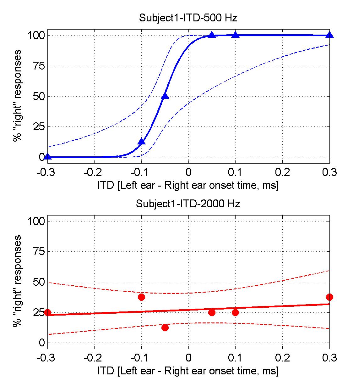
If you are doing these exercises as part of a taught class, you should again consider making a print-out of these result graphs so that you can show them to your instructors if necessary.
Using the same considerations you used when you interpreted the ILD data, answer the following questions:
Question: What is your "ITD threshold" for each of the frequencies tested?
Question: Would you consider your ITD thresholds for the two frequencies similar, or substantially different?
Evaluate the usefulness of ITDs
Evaluate the usefulness of ITDs
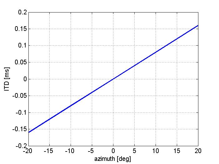
Unlike ILDs, ITDs are generally thought not to vary much with frequency. The graph below shows ITDs as a function of sound source direction measured in an adult male with small microphones inserted in the ear canal.
Question: Use the graph to work out what MAAs the ITD thresholds you have obtained would correspond to. How do these MAAs compare to those you obtained for ILDs?
Was Rayleigh correct?
Was Rayleigh correct?
Lord Rayleigh is credited for developing the "duplex theory" for sound localization, which states that the brain relies heavily on ITDs for low frequency sounds, and on ILDs for high frequency sounds.
Final Question: In your own words, do the results you have obtained in this practical agree with the duplex theory?
This concludes this practical.
(Note that this practical varied ILDs or ITDs independently, one at a time. In nature, they do of course tend to vary together, so that sounds that are louder in the left also tend to arrive earlier at the left. So how does the brian put ITDs and ILDs together? If you are curious you can explore this on the next page.)
Time intensity trading
Time intensity trading
Move the mouse cursor over the grid below to hear a harmonics complex tone with ILDs and ITDs as indicated.
You should listen to these sounds over headphones, and this demo may not work for you if you have a significant hearing loss in one ear, or if the sound card on your computer is of poor quality and does not separate the two stereo channels well. Note also that many wireless bluetooth headphones are not regenerating ITDs properly, so if you use wireless headphones this may not work either.
Positive ILDs and ITDs should make the sound appear to come from the right. Hence, the sounds toward the top right should sound the furthest right, the ones in the bottom left the furthest left. (Make sure you have your headphones on the right way around.)
The curious thing to observe here is that, if you start from the middle, you can move the sound right either by moving the mouse cursor up, or by moving it right. You change the sounds in two very different ways (in one case you change the timing between the ears, in the other you change the relative sound intensity) but although the manipulations are very different in nature, they produce the same effect: the sound appears to come from the right. Can you tell by listening carefully whether the sound percept moves because of timing or intensity cues?
Another thing to try is this: start from the middle, move the sound right by moving the cursor right, then move the cursor down. As you move the cursor down the sound should appear to move back toward the middle, because the timing and intensity cues now point in opposite directions, and your brain perceives the sound at a compromise position somewhere in between.
Binaural Beats - Sound Example
Binaural Beats - Sound Example
As discussed in the context of Figure 5-5 of "Auditory Neuroscience" (reproduced here below) ITD cues for sound location are derived from the interaural phase. Conequently, tones that are slightly mis-tuned and which are delivered separately to the left and right ear can give the impression of a shifting lateralization from left or right. THe sound example here below shows this. To the left ear we play a 500 Hz pure tone, to the right ear a 500.25 Hz pure tone. So the left and right ear go in and out of phase once every 4 seconds. The left and right ear start in phase, so when listened to over headphones, the sound should start off sounding as if it was in the middle. However, since the frequency in the right ear is ever so slightly higher (the oscillations are ever so slightly faster), over the next 2 seconds the right ear's phase starts to lead by up to 1 ms, giving a changing ITD cue that suggests that the sound is shifted to the right. After more than 2 seconds, the right ear phase leads by more than 1 ms, but since the period of the tones is 2 ms long, the brain may interpret this as a less than 1 ms phase lead in the left ear. So about 2 seconds into the demo, the sound will sound as if it is now suddenly coming from the left, but then it will gradually shift over to the right again over the next 4 seconds, only to then jump again to the left, and so forth.
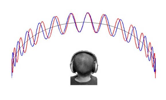
Steady pure tones are unpleasant to listen to, and they also produce a great deal of adaptation in the auditory nervous system, making it difficult to perceive them well. We therefore added a 5 Hz sinusoidal amplitude modulation to the this demo. It makes the effect easier to hear.
This demo is designed to be listened to over stereo headphones. It may not work over loudspeakers. Also, some individuals will have difficulty hearing the effect, particularly if they have a history of ear problems in either ear which may interfere with binaural hearing.
How does it work? : You can choose the frequency of the sound and select a difference between the two frequencies which make the sound. The frequency difference allows you to hear the sound as if it is moving around you. To hear this effect, select a frequency and an amplitude to make the modulation. You can press Start/Stop button to play or to end the sound.
Frequencies : Frequency: 0 2000 Difference:
Frequency 1 Value :
Hz Frequency 2 Value : HzModulation : Frequency: 0 10
Frequency Modulation Value :
HzAmplitude : Amplitude: 0 1
Amplitude Value :
Virtual Acoustic Space
Virtual Acoustic Space
The numbered squares signify the sound directions corresponding to a series of "virtual acoustic space" stimuli, which were generated by convolving a stimulus - in this case, a series of tapping sounds - with the head-related transfer function of one of the authors of this book.
Put on a pair of - preferably fairly good - headphones and plug them into the headphone socket of your computer. By moving the mouse over the squares, you will hear the stimulus changing location. Most stererophonic recordings are based only on differences in level between the two ears and the resulting sounds are therefore lateralized toward one ear or the other. By contrast, virtual acoustic space stimuli incorporate the full complement of localization cues and, in principle, replicate real free-field sounds. Consequently, as you move the mouse, you should hear the sounds move up or down as well as left or right and even seem as though they are either in front of or behind you. Of course, how well this will work depends to some extent on how closely your head and ears match those of the subject from whom the acoustical measurements were made to generate these stimuli.